Visualizing temperature anomalies with Clojure and Oz

Clojure is an oddball for a lisp. It is quite powerful and opinionated, it works well in the Java and Javascript ecosystem and has good tooling in emacs aka CIDER. For me I prefer other lisps for their more non-opinionated style but still Clojure is a wonderful tool and it seems to have a blossoming community that is really responsive to the modern computing environment. This is especially important since it offers a way for lispers to get their hands on things going on in the world of Java and Javascript without losing the developing expressiveness and experience of a lisp.

So, today I took part in a meeting organized by SciCloj, a group of people conspiring to make Clojure a powerful language for the scientific and data analysis fields. Christopher Small presented his work on Oz, a clojure wrapper around the powerful Vega/Vega Lite libraries.

The point of Vega and Oz is to create declaration of plots as data that then can be exported in different formats. This data handling sure is familiar to people that work with Clojure. So in Vega we create plots that are describers in JSON and this works with edn, the JSON-like format in Clojure, in Oz.

Let’s see a simple example: let’s visualize the annual temperature anomalies for every year after 1880 as reported from the NCDC of NOAA USA.

Personally I use the Leiningen build tool for Clojure so let’s start with creating a new project:

lein new temperature-anomalies

Then the only thing to get start is to add [metasoarous/oz “1.6.0-alpha3”] to our dependencies vector in project.clj. After that we can open our src/temperature-anomalies/core.clj file and start playing with Oz.

(ns temperature-anomalies.core
  (:require [oz.core :as oz]))

After giving a slight handling to our data we can then define:

(def temperatures
  '({:year "1939" :delta "0.01"}
    {:year "1881" :delta "-0.09"}
    {:year "1915" :delta "-0.09"}
    {:year "1904" :delta "-0.46"}
    {:year "1996" :delta "0.32"}
    {:year "2015" :delta "0.93"}
    {:year "1957" :delta "0.07"}
    {:year "1885" :delta "-0.25"}
    {:year "1998" :delta "0.65"}
    {:year "1893" :delta "-0.32"}
    {:year "1961" :delta "0.09"}
    {:year "1924" :delta "-0.24"}
    {:year "1938" :delta "-0.02"}
    {:year "1906" :delta "-0.21"}
    {:year "1942" :delta "0.11"}
    ...))

So now the main entry to Oz is the view function. Given a map that describes the plot, view starts a web server that setups the visualization. So in our example:

(def line-plot
 {:data
  {:values temperatures}
  :encoding {:x {:field "year"}
	     :y {:field "delta"}}
  :mark "line"})

  (def stacked-bar
   {:data
    {:values temperatures}
    :mark "point"
    :encoding {:x {:field "year"}
	       :y {:field "delta"}}})

  (oz/view! line-plot)

What we get is:

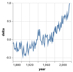
Voila, we have some nice plots to show us that anomalies in temperature get worse every year. By reading more about the Vega Lite data structure to describe plots we can find more ways to visualize our data. The example was fairly simple and doesn’t really convey the full capabilities of the tool. Some nice feature include the ability to use the visualizations is Reagent components and also a full blown static site generator. This could be nice in the case where you want to export the results of some kind of research.

Any way that’s for now and keep it up!